Warning for Sensitive Contents! This post contains photos of bugs. If you are sensitive about insects, please close the tab immediately!
Dive into Deep Learning
Lucas Zhang
Train a deep learning model to classify beetles, cockroaches and dragonflies using these images. Original images from https://www.insectimages.org/index.cfm. Explain how the neural network classified the images using SHapley Additive exPlanations.
Solution:
Please also visit my GitHub Page and GitHub repository
Train a neural network model to distinguish the three insects
Source code adapted from a tensorflow demo.
Initialization
To achieve our aims, we require packages matplotlib.pyplot, numpy, os, PIL and tensorflow.
Note: The latest version of tensorflow (2.7.0) is required for the following source code.
#Import required packages
import matplotlib.pyplot as plt
import numpy as np
import os
import PIL
import tensorflow as tf

from tensorflow import keras
from tensorflow.keras import layers
from tensorflow.keras.models import Sequential

#Import required figure
import glob
train = [f for f in glob.glob('insects/train/*/*.jpg')]
print("We have", len(train),"figures in the \'train\' folder.")
test = [f for f in glob.glob('insects/test/*/*.jpg')]
print("We have", len(test), "figures in the \'test\' folder")
It shows we have 1019 figures in the ‘train’ folder and 180 figures in the ‘test’ folder. Next, we may want to see a few example photos of beetles, cockroaches and dragonflies in our dataset.
beetles = list(glob.glob('insects/train/beetles/*.jpg'))
PIL.Image.open(str(beetles[152]))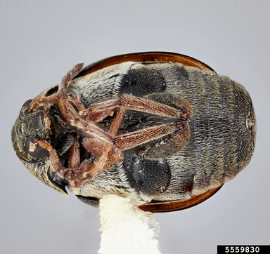
cockroaches = list(glob.glob('insects/train/cockroach/*.jpg'))
PIL.Image.open(str(cockroaches[15]))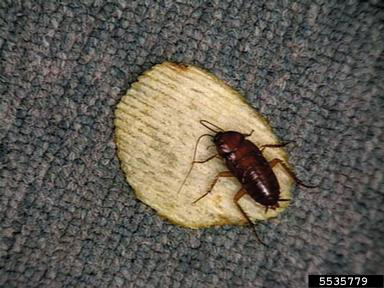
dragonflies = list(glob.glob('insects/train/dragonflies/*.jpg'))
PIL.Image.open(str(dragonflies[175]))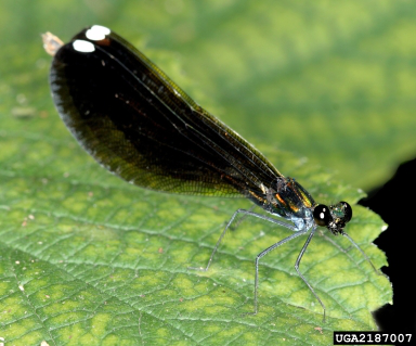
Configure the neural network model
We need to set the training dataset (using the photos in the “train” folder) and the test dataset (using the “test” folder) for our neural network model. Here we use functions in tensorflow.keras to help set up the configuration. We first set the training set and test set, and check the names of the 3 classes in our dataset.
train_ds = tf.keras.utils.image_dataset_from_directory(directory = "insects/train")
#tf.keras.utils.image_dataset_from_directory(
#    directory, labels='inferred', label_mode='int',
#    class_names=None, color_mode='rgb', batch_size=32, image_size=(256,
#    256), shuffle=True, seed=None, validation_split=None, subset=None,
#    interpolation='bilinear', follow_links=False,
#    crop_to_aspect_ratio=False, **kwargs
val_ds = tf.keras.utils.image_dataset_from_directory(directory = "insects/test")class_names = train_ds.class_names
print(class_names)We found 1021 files belonging to 3 classes in the ‘train’ folder and 187 files belonging to 3 classes in the ‘test’ folder, and these photos are [‘beetles’, ‘cockroach’, ‘dragonflies’]. Next, we display some photos in our training dataset.
import matplotlib.pyplot as plt

plt.figure(figsize=(10, 10))
for images, labels in train_ds.take(1):
  for i in range(9):
    ax = plt.subplot(3, 3, i + 1)
    plt.imshow(images[i].numpy().astype("uint8"))
    plt.title(class_names[labels[i]])
    plt.axis("off")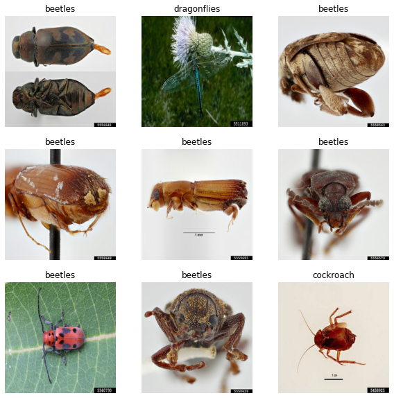
Train the neural network model
In this section, we will set up a buffer for our model, convert the color scale [0, 255] to (0, 1) scale, set up layers for the neural network model and finally, learn the parameters in our neural network model.
#this is to create buffer for our model
AUTOTUNE = tf.data.AUTOTUNE
train_ds = train_ds.cache().shuffle(1000).prefetch(buffer_size=AUTOTUNE)
val_ds = val_ds.cache().prefetch(buffer_size=AUTOTUNE)

#we convert the color value to (0, 1) scale
normalization_layer = layers.Rescaling(1./255)

#set up the layers in the neural network
num_classes = 3

model = Sequential([
  layers.Rescaling(1./255, input_shape=( 256, 256, 3)),
  layers.Conv2D(16, 3, padding='same', activation='relu'),
  layers.MaxPooling2D(),
  layers.Conv2D(32, 3, padding='same', activation='relu'),
  layers.MaxPooling2D(),
  layers.Conv2D(64, 3, padding='same', activation='relu'),
  layers.MaxPooling2D(),
  layers.Flatten(),
  layers.Dense(128, activation='relu'),
  layers.Dense(num_classes)
])

#compile the layers
model.compile(optimizer='adam',
              loss=tf.keras.losses.SparseCategoricalCrossentropy(from_logits=True),
              metrics=['accuracy'])
After these steps, we can check the properties of different layers in our neural network.
model.summary()It shows we have a total of 8,412,707 trainable parameters in our model. Thereafter, we are about to learn the parameters in the model or namely, to train the neural network.
epochs = 5
history = model.fit(
  train_ds,
  validation_data=val_ds,
  epochs=epochs
)
Quality-checking
In this section, we will exam our model using the “test” dataset. A good model should have high training accuracy and low loss, but we should also avoid over-fitting. Overfitting occurs if the model on the training set is much better than the test set.
In addition to the statistics, we will also check if our trained model can successfully identify the insect in some figures provided in the test folder or on the internet.
acc = history.history['accuracy']
val_acc = history.history['val_accuracy']

loss = history.history['loss']
val_loss = history.history['val_loss']

epochs_range = range(epochs)

plt.figure(figsize=(8, 8))
plt.subplot(1, 2, 1)
plt.plot(epochs_range, acc, label='Training Accuracy')
plt.plot(epochs_range, val_acc, label='Validation Accuracy')
plt.legend(loc='lower right')
plt.title('Training and Validation Accuracy')

plt.subplot(1, 2, 2)
plt.plot(epochs_range, loss, label='Training Loss')
plt.plot(epochs_range, val_loss, label='Validation Loss')
plt.legend(loc='upper right')
plt.title('Training and Validation Loss')
plt.show()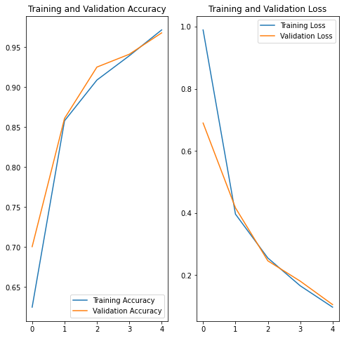
These figures show that our model works well on both training and test datasets with high accuracy and low loss. We will next test our model with some real examples, including one specific photo in our dataset and one from the internet.
dragonflies = list(glob.glob('insects/test/dragonflies/*.jpg'))
PIL.Image.open(str(dragonflies[2]))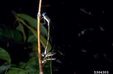
img = tf.keras.utils.load_img(str(dragonflies[2]), target_size=(256, 256))
img_array = tf.keras.utils.img_to_array(img)
img_array = tf.expand_dims(img_array, 0) # Create a batch

predictions = model.predict(img_array)
score = tf.nn.softmax(predictions[0])

print(
    "This image most likely belongs to {} with a {:.2f} percent confidence."
    .format(class_names[np.argmax(score)], 100 * np.max(score))
)
It shows “This image most likely belongs to dragonflies with a 99.85 percent confidence.” We next use a photo from the internet to test.
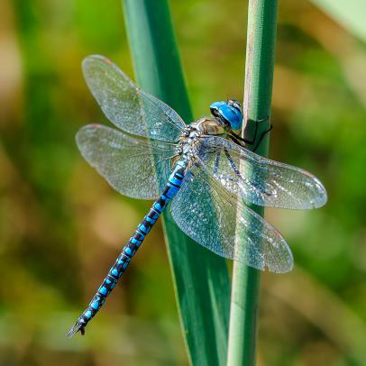
img = tf.keras.utils.load_img("dragonfly1.jpeg", target_size=(256, 256))
img_array = tf.keras.utils.img_to_array(img)
img_array = tf.expand_dims(img_array, 0) # Create a batch

predictions = model.predict(img_array)
score = tf.nn.softmax(predictions[0])

print(
    "This image most likely belongs to {} with a {:.2f} percent confidence."
    .format(class_names[np.argmax(score)], 100 * np.max(score))
)
It shows “This image most likely belongs to dragonflies with a 99.93 percent confidence.” Combining these results, it appears that our model can identify the dragonflies very well. But how does it work? We will use SHAP values to illustrate this point.
Explain our model using SHAP
In the following section, we would like to explain how our model works. We will calculate the SHAP value for a different part in one of our previous figures. Source code adapted from h1ros.
Initialization
To achieve our aims, we require packages shap, skimage.segmentation, pandas, numpy, matplotlib.pyplot and warnings.
Note: The latest version of tensorflow (2.7.0) is required for the following source code.
import shap
shap.initjs()

import keras
from skimage.segmentation import slic
import pandas as pd
import numpy as np
import matplotlib.pyplot as plt
import warnings

%matplotlib inline

# make a color map
from matplotlib.colors import LinearSegmentedColormap
colors = []
for l in np.linspace(1, 0, 100):
    colors.append((245 / 255, 39 / 255, 87 / 255, l))
for l in np.linspace(0, 1, 100):
    colors.append((24 / 255, 196 / 255, 93 / 255, l))
cm = LinearSegmentedColormap.from_list("shap", colors)

# load model data
feature_names = class_names
model = model
We will again use the dragonfly photo from the internet to calculate the SHAP values for its different parts.
# load an image
pic_str = "dragonfly1.jpeg"
img = tf.keras.utils.load_img(pic_str, target_size=(256, 256))
img_orig = tf.keras.utils.img_to_array(img)
plt.imshow(img);
plt.axis('off');

#img = tf.keras.utils.load_img(pic_str, target_size=(256, 256))
#img_array = tf.keras.utils.img_to_array(img)
#img_array = tf.expand_dims(img_array, 0) # Create a batch
#predictions = model.predict(img_array)
#score = tf.nn.softmax(predictions[0])
Divide the picture into different parts
We may want to divide the picture into different parts to see which part plays an important role in our model.
# Create segmentation to explain by segment, not every pixel
n_segments = 100
segments_slic = slic(img, n_segments = n_segments, compactness = 5, sigma= 3)
plt.imshow(segments_slic);
plt.axis('off');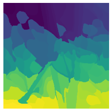
Set up the SHAP kernel explainer and calculate the SHAP value
We will calculate the SHAP value by blocking specific parts and observing how the model outcome may change.
# define a function that depends on a binary mask representing if an image region is hidden
def mask_image(zs, segmentation, image, background=None):

    if background is None:
        background = image.mean((0, 1))

    # Create an empty 4D array
    out = np.zeros((zs.shape[0],
                    image.shape[0],
                    image.shape[1],
                    image.shape[2]))

    for i in range(zs.shape[0]):
        out[i, :, :, :] = image
        for j in range(zs.shape[1]):
            if zs[i, j] == 0:
                out[i][segmentation == j, :] = background
    return out


def f(z):
    return model.predict(mask_image(z, segments_slic, img_orig, 255))
#img = tf.keras.utils.load_img(pic_str, target_size=(256, 256))
#img_array = tf.keras.utils.img_to_array(img)
#img_array = tf.expand_dims(img_array, 0) # Create a batch
#predictions = model.predict(img_array)

def fill_segmentation(values, segmentation):
    out = np.zeros(segmentation.shape)
    for i in range(len(values)):
        out[segmentation == i] = values[i]
    return out

masked_images = mask_image(np.zeros((1, n_segments)), segments_slic, img_orig, 255)

plt.imshow(masked_images[0][:,:, 0]);
plt.axis('off');
We calculate the SHAP values for each part.
# use Kernel SHAP to explain the network's predictions
explainer = shap.KernelExplainer(f, np.zeros((1, n_segments)))

with warnings.catch_warnings():
    warnings.simplefilter("ignore")
    shap_values = explainer.shap_values(np.ones((1, n_segments)), nsamples=300) # runs model 300 times
Visualize the SHAP for different parts in the photo
Finally, we are able to examine which part in our previous example contributes more to the model result.
#Get the output
predictions = model.predict(np.expand_dims(img_orig.copy(), axis=0))
top_preds = np.argsort(-predictions)

# Visualize the explanations
fig, axes = plt.subplots(nrows=1, ncols=4, figsize=(12,4))
inds = top_preds[0]
axes[0].imshow(img)
axes[0].axis('off')

max_val = np.max([np.max(np.abs(shap_values[i][:,:-1])) for i in range(len(shap_values))])
for i in range(3):
    m = fill_segmentation(shap_values[inds[i]][0], segments_slic)
    axes[i+1].set_title(feature_names[inds[i]])
    axes[i+1].imshow(np.array(img.convert('LA'))[:, :, 0], alpha=0.15)
    im = axes[i+1].imshow(m, cmap=cm, vmin=-max_val, vmax=max_val)
    axes[i+1].axis('off')
cb = fig.colorbar(im, ax=axes.ravel().tolist(), label="SHAP value", orientation="horizontal", aspect=60)
cb.outline.set_visible(False)
plt.show()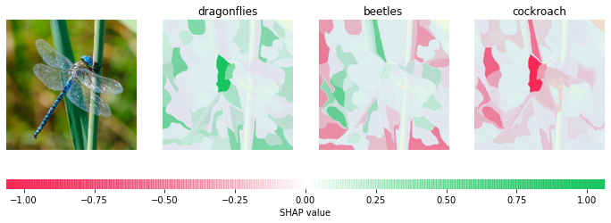
pd.Series(data={feature_names[inds[i]]:predictions[0, inds[i]] for i in range(3)}).plot(kind='bar', title='Predictions');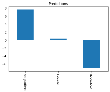
It shows our model correctly predicts the photo as dragonflies with a high score. This prediction is partially because the background and the middle part of the body make it look like a “dragonfly”